intro

Variational autoencoders (VAEs) are a type of generative model. Variational homoencoders were introduced in this paper and extend the idea of VAEs by providing amortized class information.

background

vae

For background on the VAE see this post.

One problem with VAEs is that, with a sufficiently powerful decoder, they can learn to ignore the latent codes. The MDL says that if we can use the least number of bits then we have achieved the best hypothesis for the data. If the decoder learns to ignore $z$ and just learns $p(X)$ then $q(z|x)$ can just learn $p(z)$. This can happen at the beginning of training when the approximate posterior ($q$) doesn’t produce meaningful information on $x$. The optimization routine then just attempts to make $q$ equal to the prior ($p(z)$). As $H(X)$ is the optimal possible compression for $X$, meaningful latent codes will never be learned.

vhe

One solution to this problem is to amortize the cost of sending class level information over many samples. From the paper:

$\begin{align} C_{total} &= \mathop{\mathbb{E}}_{\substack{x \in X \\ D \subset X_x}} \left[ \mathop{\mathbb{E}}_{\substack{q \left( c|D \right) \\ q \left( z|c, x \right)}} \left[ \log{ p \left( x | c, z \right) } + D_{KL} \left( q \left( z | c, x \right) || p \left( z|c \right) \right) + \frac{1}{|X_x|} D_{KL} \left( q \left( c | D \right) || p \left( c \right) \right) \right] \right] \end{align}$

This amounts to the following training algorithm:

Pick a training example $x$.
Pick a subset $D$ that has the same label as $x$.
Encode $D$ to get $c$.
Encode $x$ conditioned on $c$ to get $z$.
Reconstruct $x$ from $c$ and $z$.

Ideally $c$ will encode information about the class whereas $z$ will encode information about how $x$ delivers from its class.

kl divergence derivation

See this post.

unsupervised VHEs

There is a comparitive dearth of supervised data so an important question becomes how to extend algorithms like this into the unsupervised regime. I posit that we can get pseudo-labels (or at least a meaningful measure of proximity) using the latent codes produced by $q \left( c | D \right)$ and $q \left( z | c, x \right)$. From here on I will refer to a code as the concatenation of the class code and individual example code.

By using a clustering algorithm on the codes we can get an idea of how similar two training examples are. At the beginning of training, the similarity will be dominated by the $z$ portion of the code since $D$ will be chosen basically at random. The function $q \left( z | c, x \right)$ will effectively ignore $c$ and just encode $x$ like a typical VAE. As training progresses, however, the $D$s become more representative of the training example since examples with similar $z$ codes will be chosen. The $c$ parts of the codes then become more meaningful and $z$s start encoding differences.

The training algorithm looks the same as before with the following differences:

Initialization:

Pick codes from $N(0, 1)$ for every training example $x$.
Initialize a KMeans clustering algorithm with codes.

Before each epoch:

Associate each training example with labels based on the clustering.

Training:

Record the new values of $z$ and $c$ for this $x$.

code

The full code is available on GitHub.

vae

The following code implements the distributions required for equation 1.

class VHE(nn.Module):

    def __init__(self, code_len):

        super().__init__()

        self.encode_c_u = nn.Sequential(
            nn.Linear(28 * 28, 512),
            nn.ReLU(True),
            nn.Linear(512, code_len),
        )

        self.encode_c_logstd = nn.Sequential(
            nn.Linear(28 * 28, 512),
            nn.ReLU(True),
            nn.Linear(512, code_len),
        )

        self.encode_z_u = nn.Sequential(
            nn.Linear(28 * 28 + code_len, 512),
            nn.ReLU(True),
            nn.Linear(512, code_len),
        )

        self.encode_z_logstd = nn.Sequential(
            nn.Linear(28 * 28 + code_len, 512),
            nn.ReLU(True),
            nn.Linear(512, code_len),
        )

        self.prior_z_mu = nn.Sequential(
            nn.Linear(code_len, 512),
            nn.ReLU(True),
            nn.Linear(512, code_len),
        )

        self.prior_z_logstd = nn.Sequential(
            nn.Linear(code_len, 512),
            nn.ReLU(True),
            nn.Linear(512, code_len),
        )

        self.decode_cz = nn.Sequential(
            nn.Linear(2 * code_len, 512),
            nn.ReLU(True),
            nn.Linear(512, 28 * 28),
            nn.Sigmoid(),
        )

And here is how those distributions are used:

def forward(self,
            inputs: torch.Tensor,
            inputs_class: torch.Tensor):

    # mean to get from N x D x H * W to N x H * W
    u = self.encode_c_u(inputs_class)
    mean = u.mean(dim=0)
    logstd = self.encode_c_logstd(inputs_class).mean(dim=0)
    q_c = NormalParams(mean, logstd)
    c_sample = self.reparametrize(q_c.u, q_c.s)

    # condition the posterior of z on c
    inputs_augmented = torch.cat([inputs, c_sample], dim=-1)

    # N x H * W + CODE_LEN
    q_z = NormalParams(self.encode_z_u(inputs_augmented), self.encode_z_logstd(inputs_augmented))
    z_sample = self.reparametrize(q_z.u, q_z.s)

    p_c = NormalParams(torch.tensor(0, dtype=torch.float32), torch.tensor(0, dtype=torch.float32))
    p_z = NormalParams(self.prior_z_mu(c_sample), self.prior_z_logstd(c_sample))

    latent = torch.cat([z_sample, c_sample], dim=1)

    output = self.decode_cz(latent)

    return output, q_c, p_c, q_z, p_z

where NormalParams is just a wrapper for mean u and log standard deviation s:

from collections import namedtuple

NormalParams = namedtuple('NormalParams', ['u', 's'])

def calc_loss(x: torch.Tensor,
              recon: torch.Tensor,
              cardinality_class: torch.Tensor,
              params_q_c: NormalParams,
              params_p_c: NormalParams,
              params_q_z: NormalParams,
              params_p_z: NormalParams) -> torch.Tensor:
    # reconstruction
    xent = F.binary_cross_entropy(recon, x, size_average=False)

    # class coding cost
    dkl_c = dkl_2_gaussians(params_q_c, params_p_c, weights=1 / cardinality_class)

    # sample coding cost
    dkl_z = dkl_2_gaussians(params_q_z, params_p_z)

    return xent + dkl_c + dkl_z

def dkl_2_gaussians(q: NormalParams,
                    p: NormalParams,
                    weights: torch.Tensor = None) -> torch.Tensor:

    dkls = p.s - q.s - 0.5 + ((2 * q.s).exp() + (q.u - p.u).pow(2)) / (2 * (2 * p.s).exp())

    if weights is not None:
        dkls *= weights[:, None]

    dkl = torch.sum(dkls)

    return dkl

results

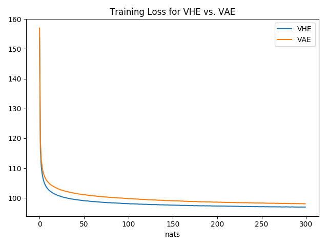
The following results correspond to two layer simple feedforward (512 dimensional hidden layer) architectures for both the VAE and the unsupervised VHE. Note that the VHE actually has more parameters since it has two encoding networks.

loss

The following shows the average loss (in nats) for each training epoch. We see that amortizing information transfer using a pseudo-class does result in fewer nats used.

Losses VAE VHE

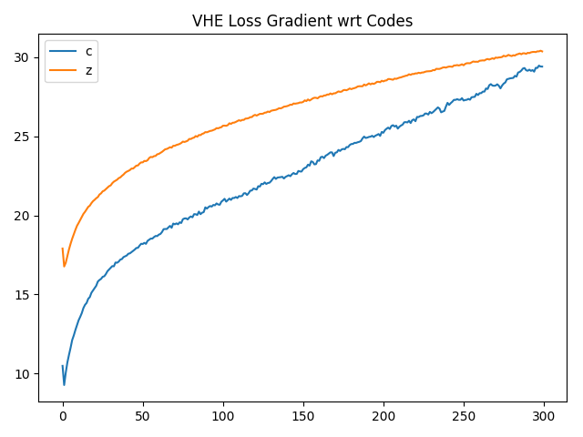
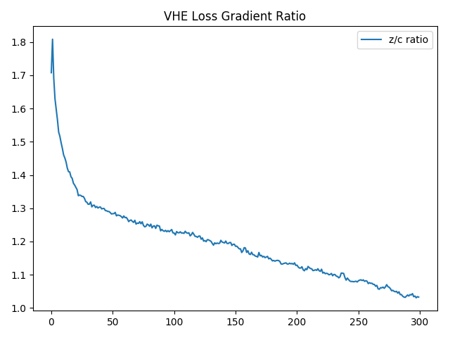
z & c contributions

Given the class labels are initially chosen at random (since class codes are initially randomized) we would expect the contribution from the $c$ component of the latent code to be meaningless at the start of training. As the $z$ components of the latent codes begin to cluster then the membership of this cluster can be learned by the $c$ component of the code. This relationship is something that we notice when looking at the derivative of the loss with respect to each of the two components:

VHE Gradients z c

VHE Gradient Ratio z:c

future work

Clearly using the l2 norm on the codes does not provide for an optimal balance between the $c$ and $z$ components. Importantly the $z$ component will eventually prevent some examples from the same class from being labeled as such. This occurs when the model does a good job at discriminating between classes but the $z$ distributions force them into separate clusters. Below are a few ideas of solutions:

Anneal weights applied to $c$ and $z$ over the course of training. This is problematic because it is not a universal solution.
Calculate weights applied to $c$ and $z$ as a function of their respective loss gradients. Again this does not seem necessarily easily generalizeable.
Use estimates of the mutual information between latent codes and the input to determine these weights.

additional resources

The original paper
All the code used in this post can be found on GitHub.
Associative Compression Networks (another solution to this problem)