intro

Variational autoencoders (VAEs) are a type of generative model. Associative compression networks were introduced in a paper by Alex Graves and extend the idea of VAEs by ordering the training data.

background

vae

There are a couple equivalent ways of looking at VAEs.

Information theory
Variational lower bound

Terms:

$p(z {\vert} x)$ the true optimal posterior distribution
$q(z {\vert} x)$ given by the encoder (an approximation of the true posterior distribution)
$p(z)$ the prior distribution over the latent space
$p(x {\vert} z)$ reconstruction probability given by the decoder

information theory

We calculate the the total number of bits to transmit a message. The minimum description length principle (MDL) says that the best description (model) of a dataset is the one that can compress the data the best. So if we can reduce the number of bits required to compress a dataset we can find a good model of the data.

Bits to reconstruct $x$ from $z$:

$\begin{align} C_{recon} &= \int{q(z {\vert} x) \log{\frac{1}{p(x {\vert} z)}} dx} \\ &= H(q, p) \end{align}$

Bits to encode $z$ with a rebate of bits (information) from the choice of $z$:

$\begin{align} C_{coding} &= \int{q(z {\vert} x) \log{ \frac {1} {p(z)} dx}} - \int{q(z {\vert} x) \log{ \frac {1} {q(z {\vert} x)} } dx} \\ &= D_{KL}(q(z {\vert} x) || p(z)) \end{align}$

The sum of the $C_{recon}$ and $C_{coding}$ represents the total number of bits to transmit our dataset $X$ under our model posterior distribution $q(z {\vert} x)$ and model reconstructive distribution $p(x {\vert} z)$:

$C_{total} = H(q(z {\vert} x), p(x {\vert} z)) + D_{KL}(q(z {\vert} x) || p(z))$

variational lower bound

We want to come up with a distribution $q(z)$ that estimates our true posterior $p(z {\vert} x)$ (since it is difficult to compute this).

$\begin{align} D_{KL}(q(z) || p(z {\vert} x)) &= E_{z {\sim} q(z)} [ \log{q(z)} - \log{p(z {\vert} x)} ] \\ &= E_{z {\sim} q(z)} [ \log{q(z)} - \log{p(x {\vert} z)} - \log{p(z)} + \log{p(x)} ] \\ &= D_{KL}(q(z {\vert} x) || p(z)) + H(q(z {\vert} x), p(x {\vert} z)) + \log{p(x)} \\ \end{align}$

There are a couple interpretations of this last form:

$D_{KL}$: Minimizing the KL divergence amounts to minimizing the first two terms (since $\log{p(x)}$ is constant under our optimization)

ELBO: Since $D_{KL}$ is non-negative we get:

$\log{p(x)} \ge -D_{KL}(q(z {\vert} x) || p(z)) + -H(q(z {\vert} x), p(x {\vert} z))$

The right hand side forms an “evidence based lower bound” (ELBO) and by maximizing it, we maximize the probability of our data.

problem

One problem with VAEs is that, with a sufficiently powerful decoder, they can learn to ignore the latent codes. The MDL says that if we can use the least number of bits then we have achieved the best hypothesis for the data. If the decoder learns to ignore $z$ and just learns $p(X)$ then $q(z|x)$ can just learn $p(z)$. This can happen at the beginning of training when the approximate posterior ($q$) doesn’t produce meaningful information on $x$. The optimization routine then just attempts to make $q$ equal to the prior ($p(z)$). As $H(X)$ is the optimal possible compression for $X$, meaningful latent codes will never be learned.

acn

One thing you may have noticed in the VAE is that the prior is just a distribution in the latent space ($p(z)$). This is typically modelled using a multivariate standard Gaussian distribution. There’s nothing that says the prior needs to be a marginal distribution. The key insight of this paper is to realize that we can order the data and then condition the prior distribution on the latent variable for the previous datum. This addresses the VAE problem since each latent code for a datum informs the distribution over the next latent code. Thus transmitting the common characteristics of a segment of data is amortized over that segment.

The question then becomes how should we order the data? We compare similarity in the latent space (initialized randomly). When an input is encoded, we can look at codes that are close to the encoded input and choose one. By choosing a unique code (and therefore datum) for each example in an epoch we choose an orderding for the data.

KL derivation

Since we are using a nonstandard Gaussian distribution for our prior (as parameterized by the prior network) we can’t just use the VAE loss. Let’s calculate the KL divergence between two Gaussians.

$D_{KL}(q || p) = H(q, p) - H(q)$

Solving for the cross entropy first with $\left< \cdots \right>_q$ being the expecation under $q$:

$\begin{align} H(q, p) &= - \left< \log \left( \frac{1}{\sigma_p \sqrt {2 \pi}} \, \exp \left( \frac{\left( -x - \mu_{p} \right) ^ 2}{2 \sigma_p^2} \right) \right) \right>_q \\ &= \frac{1}{2} \log \left( \sigma_p^2 2 \pi \right) + \left< \frac{x^2 - 2 \mu_p x + \mu_p^2}{2 \sigma_p^2} \right>_q \\ &= \frac{1}{2} \log \left( \sigma_p ^ 2 2 \pi \right) + \frac{\sigma_q^2 + \mu_q^2 - 2 \mu_p \mu_q + \mu_p^2}{2 \sigma_p^2} \\ &= \frac{1}{2} \log \left( \sigma_p ^ 2 2 \pi \right) + \frac{\sigma_q^2 + \left( \mu_q - \mu_p \right) ^ 2}{2 \sigma_p^2} \\ \end{align}$

By substituting in $q$ for $p$ in the equation above, $H(q)$ is trivial:

$\begin{align} H(q) &= \frac{1}{2} \log \left( \sigma_q ^ 2 2 \pi \right) + \frac{1}{2} \end{align}$

Combining the two:

$\begin{align} D_{KL}(q || p) &= H(q, p) - H(q) \\ &= \frac{1}{2} \log \left( \sigma_p ^ 2 2 \pi \right) + \frac{\sigma_q^2 + \left( \mu_q - \mu_p \right) ^ 2}{2 \sigma_p^2} - \frac{1}{2} \log \left( \sigma_q ^ 2 2 \pi \right) - \frac{1}{2} \\ &= \log \left( \frac{\sigma_p}{\sigma_q} \right) + \frac{\sigma_q^2 + \left( \mu_q - \mu_p \right) ^ 2}{2 \sigma_p^2} - \frac{1}{2} \end{align}$

code

The full code is available on GitHub.

vae

The following code computes means and variances for a multivariate normal distribution (the encode function). It draws from that distribution and decodes the draw.

def forward(self, inputs: torch.Tensor):

    u, logstd = self.encode(inputs)
    h2 = self.reparametrize(u, logstd)
    output = self.decode(h2)

    return output, u, logstd

acn

This code in the prior network picks a unique code (that lives in latent space) for each code that we get from the VAE. In this way, the “close neighbor” code corresponds to the datum that immediately preceeds the current datum.

def forward(self, codes: torch.Tensor):

    previous_codes = [self.pick_close_neighbor(c) for c in codes]
    previous_codes = torch.tensor(previous_codes)

    return self.encode(previous_codes)

In order to pick a close neighbor in latent space we can use a K nearest neighbors model and select randomly from the K results. Because each preceeding code must be unique (across the training epoch) we resize the KNN model as needed.

def pick_close_neighbor(self, code: torch.Tensor) -> torch.Tensor:

    neighbor_idxs = self.knn.kneighbors([code.detach().numpy()], return_distance=False)[0]

    valid_idxs = [n for n in neighbor_idxs if n not in self.seen]

    if len(valid_idxs) < self.k:

        codes_new = [c for i, c in enumerate(self.codes) if i not in self.seen]
        self.fit_knn(codes_new)

        return self.pick_close_neighbor(code)

    neighbor_codes = [self.codes[idx] for idx in valid_idxs]

    if len(neighbor_codes) > self.k:
        code_np = code.detach().numpy()
        neighbor_codes = sorted(neighbor_codes, key=lambda n: ((code_np - n) ** 2).sum())[:self.k]

    neighbor = random.choice(neighbor_codes)

    return neighbor

The loss is a straightforward implementation of the derivation above (in this case s_q and s_p are log standard deviations to prevent taking the log of a negative number):

def calc_loss(x, recon, u_q, s_q, u_p, s_p):

    # reconstruction
    xent = F.binary_cross_entropy(recon, x, size_average=False)

    # coding cost
    dkl = torch.sum(s_p - s_q - 0.5 +
                    ((2 * s_q).exp() + (u_q - u_p).pow(2)) /
                    (2 * (2 * s_p).exp()))

    return xent + dkl

results

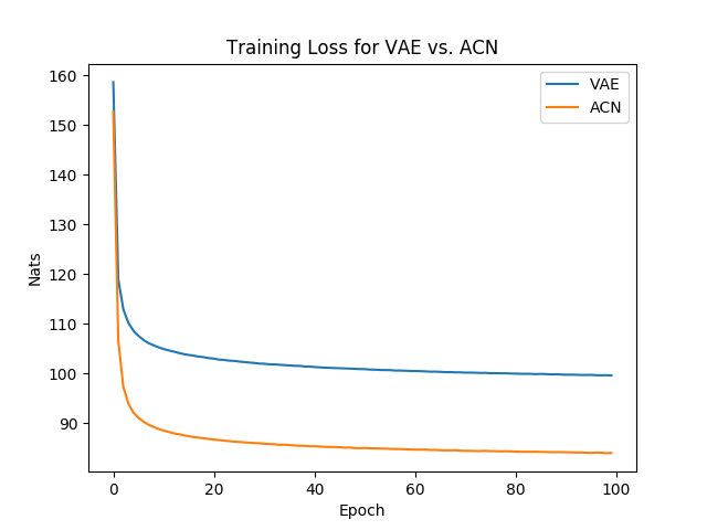
The following results correspond to two layer simple feedforward (512 dimensional hidden layer) architectures for both the VAE and the prior distribution on the MNIST dataset.

loss

The following shows the average loss (in nats) for each training epoch. We see that conditioning the prior results in a steep decrease in the number of nats required.

Losses VAE ACN

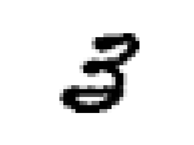
daydreaming

As discussed in the original paper we can use the prior network to “daydream”. The iterative procedure is as follows:

Encode image x using the VAE
Run the prior network on this encoding
Decode the results from the prior network using the VAE

Here is a sequence of images from a MNIST seeded daydream:

Daydreaming ACN

additional resources

The original paper by Alex Graves
All the code used in this post can be found on GitHub.