background

motivation

Markov Chain Monte Carlo (MCMC) is used when we want to estimate parameters given some data. In the Bayesian framework:

where

The problem is that the joint distribution in the denominator, $\int_{\Theta} p(X, \theta) d \theta$, can be extremely difficult to compute. If, for example, $X$ is how long a bunch of people have lived, then how might we know how often different parameters, $\theta$ occur with this dataset?

mcmc

idea

The idea of MCMC is to use a Markov chain to step through different parameter values. If the equilibrium distribution for the Markov chain equals the distribution we are trying to estimate, then we can just run the Markov chain to sample from the distribution.

metropolis hastings

derivation

One common method for doing this is called the Metropolis Hastings algorithm. If we assume a reversible Markov chain, we get the existence of an equilibrium distribution as a weaker statement. A reversible Markov chain is one that has the property of detailed balance:

where $\theta$ represents the current parameterization and $\theta’$ represents a new parameterization.

The Metropolis Hastings algorithm says we can come up with a new parameterization in two steps.

1. Generate a proposal parameterization $Q \left( \theta’ | \theta \right)$
2. Decide whether to accept or deny this proposal with probability $A \left( \theta’ | \theta \right)$ (called the acceptance ratio)

This means:

From detailed balance we get:

One solution to this is:

This works but notice that the $P \left( \theta’ \right)$ and $P \left( \theta \right)$ terms correspond to the true distribution over parameters. Because we don’t have access to this distribution, we should really have used $P \left( \theta’ | X \right)$ and $P \left( \theta | X \right)$. Using Bayes rule:

where $P \left( \theta’ \right)$ and $P \left( \theta \right)$ are priors over $\theta$ and $\theta’$ respectively.

So

algorithm

Start with a random guess for parameters $\theta$.

Iterate through the following steps:

1. Generate proposal $\theta’$ with distribution $Q \left( \theta’ | \theta \right)$
2. Accept this proposal with probability $A \left( \theta’, \theta \right)$
3. Record current parameter

Use the recorded parameters as simulated draws from the posterior $P( \theta | X )$.

code

In the code below log probabilities are used to prevent floating point precision issues. A standard normal prior over parameters and a unit variance normal model are assumed. The proposal function selects a proposed update from a normal distribution centered at the current value.

import numpy as np
from matplotlib import pyplot as plt
from scipy import stats

def proposal(x, sigma=0.5):
    """
    Propose new parameters.
    """

    x_next = stats.norm(x, sigma).rvs(size=x.shape)

    return x_next


def log_likelihood(data, mu, sigma=1):
    """
    Calculate the log likelihood of some data assuming a normal distribution.
    """

    log_prob = np.log(stats.norm(mu, sigma).pdf(data)).sum()

    return log_prob


def log_prior(parameter, mu=0, sigma=1):
    """
    Calculate the log probability of some parameter assuming a normal prior distribution on that parameter.
    """

    log_probs = np.log(stats.norm(mu, sigma).pdf(parameter))

    return log_probs

def metropolis_hastings(data, n_iterations=1000):
    """
    Calculate the posterior distribution for parameters given some data.
    """

    x_current = proposal(np.ones(1))
    ll_current = log_likelihood(data, x_current)
    log_prior_current = log_prior(x_current)

    posteriors = [x_current]

    for i in range(n_iterations):

        x_proposal = proposal(x_current)
        ll_proposal = log_likelihood(data, x_proposal)
        log_prior_proposal = log_prior(x_proposal)

        accept = np.log(np.random.rand()) < ll_proposal + log_prior_proposal - ll_current - log_prior_current

        if accept:
            x_current, ll_current = x_proposal, ll_proposal

        posteriors.append(x_current)

    return posteriors

results

We can generate some fake data from a normal distribution centered at 0.5 with unit variance:

np.random.seed(0)

data = np.random.randn(1000) + 0.5

print(data.mean(), data.std())

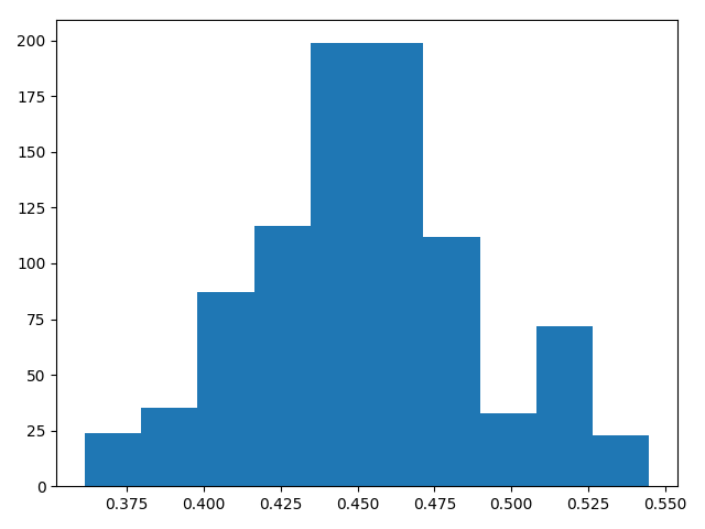
Here the actual data has mean 0.45.

And here is a histogram of draws from the posterior distribution of the mean given the data using Metropolis Hastings:

posteriors = metropolis_hastings(data)

plt.hist([x[0] for x in posteriors[100:]])
plt.show()

additional resources

• Paper on Hamiltonian Monte Carlo for intuitions behind MCMC methods and why Metropolis Hastings might fail in some cases.
• All the code used in this post can be found on GitHub.
• That said if you actually want to use MCMC in Python you should probably use an existing library (e.g. PyMC).