intro

While attempting to learn optimal optimizers I came across a slew of problems and started wondering if a sensible initialization could help. One obvious initialization is a net that has learned to imitate an existing optimizer (e.g. simple SGD, Adam, Adadelta). This post will cover the feasibility of exactly that.

Feel free to checkout the code.

background

Different optimizers use various approaches to smooth out the learning process. Techniques include momentum and second order estimation. In this post I will attempt to replicate the stochastic gradient descent optimizer with a fixed learning rate. This framework is theoretically extensible to more complicated optimizers but doing so introduces instabilities.

Stochastic gradient descent works by computing the error derivatives on a small(ish) batch of data and updating the weights accordingly. Momentum keeps track of past gradient updates and tempers future gradient updates by a decaying average of the past gradients. This increases stability by preventing a minimal number of wonky training examples from throwing off the error minimization trajectory. I will not use momentum for two reasons. Firstly it can be difficult to imitate. Secondly my intent is to get a reasonable initialization for another neural network. Other more complex features of optimizers can be learned by that neural net.

setup

There are two basic entities: models and meta-optimizers. Models will be used to generate gradients and weight updates according to an explicit optimizer (e.g. SGD). Meta-optimizers will take as input these gradients (and optionally the weight updates) and attempt to emulate the weight updates. The meta-optimizer is a recurrent neural network that uses it’s recurrence relation to infer the structure explicitly captured by the optimizer.

Note: If weight updates are passed to the meta-optimizer, they are used in a non-trivial backwards-looking manner. In other words the meta-optimizer predicted weight update at time $t$ will use the ground truth weight updates from the model at time $t-1$. This can be used to prevent distributional drift and increase training stability.

code

The full code is available on GitHub.

meta-optimizer

The following code computes weight updates for the model, defines a loss, and updates its own weights to more accurately imitate the model’s optimizer:

model = CONFIG.model_class()

grads, deltas_opt, model_losses = model.step()

truth = deltas_opt if CONFIG.supply_truth else None
deltas_pred, _ = self(grads, truth=truth)

perc_error = (deltas_opt - deltas_pred) / (deltas_opt + STABILITY)
loss = perc_error.norm()

self.zero_grad()
loss.backward()

self.optimizer.step()

model

The following code lives in the .step() method called above. It collects weight updates that the model’s optimizer performs. These are the inputs to the meta-optimizer.

for t in range(CONFIG.num_steps_model):
    inp, targets = next(self.data_gen_train)

    if isinstance(inp, np.ndarray):
        inp = torch.from_numpy(inp).float()
    if isinstance(targets, np.ndarray):
        targets = torch.from_numpy(targets).float()

    out = self(inp)

    loss = self.criterion(out, targets)

    losses.append(loss)

    self.zero_grad()
    loss.backward()

    grads.append([p.grad.clone() for p in self.params])

    params0 = [p.clone() for p in self.params]

    self.optimizer.step()
    deltas.append([p1 - p0 for (p1, p0) in zip(self.params, params0)])

results

Here are the test results we see after training a meta-optimizer to imitate stochastic gradient descent on a convolutional neural net learning the MNIST dataset. The ground truth was not supplied to the meta-optimizer and no momentum was used in the model’s optimizer.

SGD Imitator

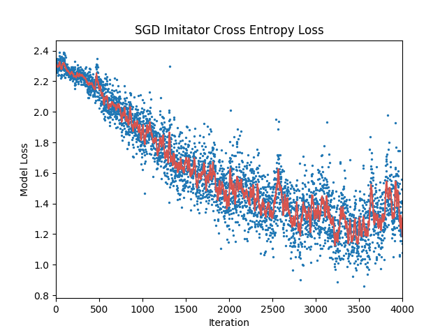
Blue dots represent actual model losses at various training steps. The red curve is a smoothed version.

Because there is only one correct classification (digit label) for any input, most of the true probabilities for labels ($p_i$) are 0. Cross entropy is then calculated as follows for the true classification distribution $p$ and the model predicted distribution $q$:

$\begin{align} xent &= -\sum{p_i \ln{q_i}} \\ &= -1 \ln{q_j} \\ &= -\ln{q_j} \end{align}$

where $j$ denotes the index of the correct classification.

If we were to guess randomly we would assign a 1/10 probability to each of the labels (0-9). So the $xent$ for a random guesser would be:

$\begin{align} xent_{rand} &= -\ln{ \frac{1}{10} } \\ &\approx 2.30 \end{align}$

Looking at the figure we can see that the model starts out guessing roughly uniformly (since $xent$ is approximately 2.30) and learns a more accurate model using the meta-optimizer. We can solve for the probability the model guesses correctly after training using the final cross entropy value of approximately 1.3:

$\begin{align} 1.3 &= 1 \ln{\frac{1}{p}} \\ p &= e^{-1.3} \\ p &\approx 27.25% \end{align}$

Clearly one thing that messes with the long term stability and accuracy is that the meta-optimizer is trained on gradient trajectories that are only 5 timesteps long (in this training run). At evaluation time, however, the meta-optimizer computes weight updates out to 4000 timesteps. This means that for the majority of the timesteps, errors are allowed to compound (in hidden states and outputs) in ways unseen at training time. This also explains the ping-ponging we see in the cross-entropy towards the end of training.