intro

Dataset Aggeregation (Dagger) is an algorithm that is used to correct distributional drift in imitation learning models. It is a great technique if the problem domain is conducive to ad-hoc data labeling (and you have the resources to do so). Dagger has four steps assuming you start with a dataset D that contains a set of observations and actions (inputs and outputs):

1. Train your model M on D.
2. Generate new paths by using M to generate an action for an output and feeding that back into M.
3. Create a new dataset D’ that consists of the observations from these new paths but actions that are supplied by an expert (e.g. a human).
4. Store D <- D’

Iterating through this means that the dataset grows to provide explicit examples that correct drift between M and the expert.

In this post we’ll examine the difference that training with Dagger can make in optimizing M. Feel free to checkout the code.

setup

We are going to use openai gym to generate our original dataset D and subsequently act as the expert. You can read more about how to generate data. The basic idea though is that the gym has a few environments. Each environment will accept some actions as input and return a few things (observations, reward, and a done flag). For example I could say I want to move left (0) or right (1) by calling the environment function with those values. Then the environment would return:

1. Observations (maybe my new perspective from this position and my new momentum)
2. Reward (maybe the number of mangos at this new position)
3. done to let us know if our simulation has ended (e.g. we’ve gone through too many timesteps or we stepped into a mangoless pit)

In this post we’ll use the environments and environement-specific experts that open ai provides to generate D and D’.

Here is the code we use to generate data. policy_fn is our expert and action_fn is the model we have built to imitate the expert policy (needed to generate D’).

def _get_data(policy_fn, env, action_fn=None, num_rollouts=20, max_timesteps=1000, render=False):

    mc_states = []

    for i in range(num_rollouts):

        obs = env.reset()

        for j in range(max_timesteps):
            action = policy_fn(obs[None, :])
            mc_states.append((obs, action[0]))

            if action_fn:
                action = action_fn(obs)
            obs, r, done, debug = env.step(action)

            if done:
                break

            if render:
                env.render()

    return mc_states

model

A relatively simple feed forward neural net is enough to show the difference between Dagger and the baseline cases. I’ve got one fully connected hidden layer with 10 neurons (relu activation).

def build_supervised_model(optimizer_name, env):

    dim_obs = env.observation_space.shape[0]
    dim_action = env.action_space.shape[0]

    inputs = tf.placeholder(tf.float32, shape=[None, dim_obs], name='observation')

    fc1 = tf.contrib.layers.fully_connected(inputs, 10, weights_regularizer=tf.contrib.layers.l2_regularizer(scale=0.1))

    fc2 = tf.contrib.layers.fully_connected(fc1, dim_action, activation_fn=tf.tanh, weights_regularizer=tf.contrib.layers.l2_regularizer(scale=0.1))

    outputs = tf.identity(fc2, name='outputs')

    targets = tf.placeholder(tf.float32, shape=[None, dim_action], name='actions')

    unreg_loss = tf.nn.l2_loss(targets - outputs, name='unreg_loss')

    reg_losses = tf.reduce_sum(tf.get_collection(tf.GraphKeys.REGULARIZATION_LOSSES), name='reg_loss')
    loss = tf.add(unreg_loss, reg_losses, name='loss')

    tf.summary.scalar('l2_reg_loss', loss)

    if optimizer_name == 'adadelta':
        opt = tf.train.AdadeltaOptimizer()
    elif optimizer_name == 'adam':
        opt = tf.train.AdamOptimizer()
    else:
        raise ValueError('Unknown optimizer name {}'.format(optimizer_name))

    update = opt.minimize(loss, name='update')

    return inputs, targets, outputs, loss, update

results

In order to get a fair comparison I limited the number of observations (\(10^8\)) seen by the Dagger model to be equal to the number seen by the baseline model.

Here is a video of the baseline model acting in the world:

And here is a video of the model trained with Dagger acting in the world:

The one trained with Dagger is clearly more robust.

Here are the average rewards and average number of actions made by the two models at different training iterations.

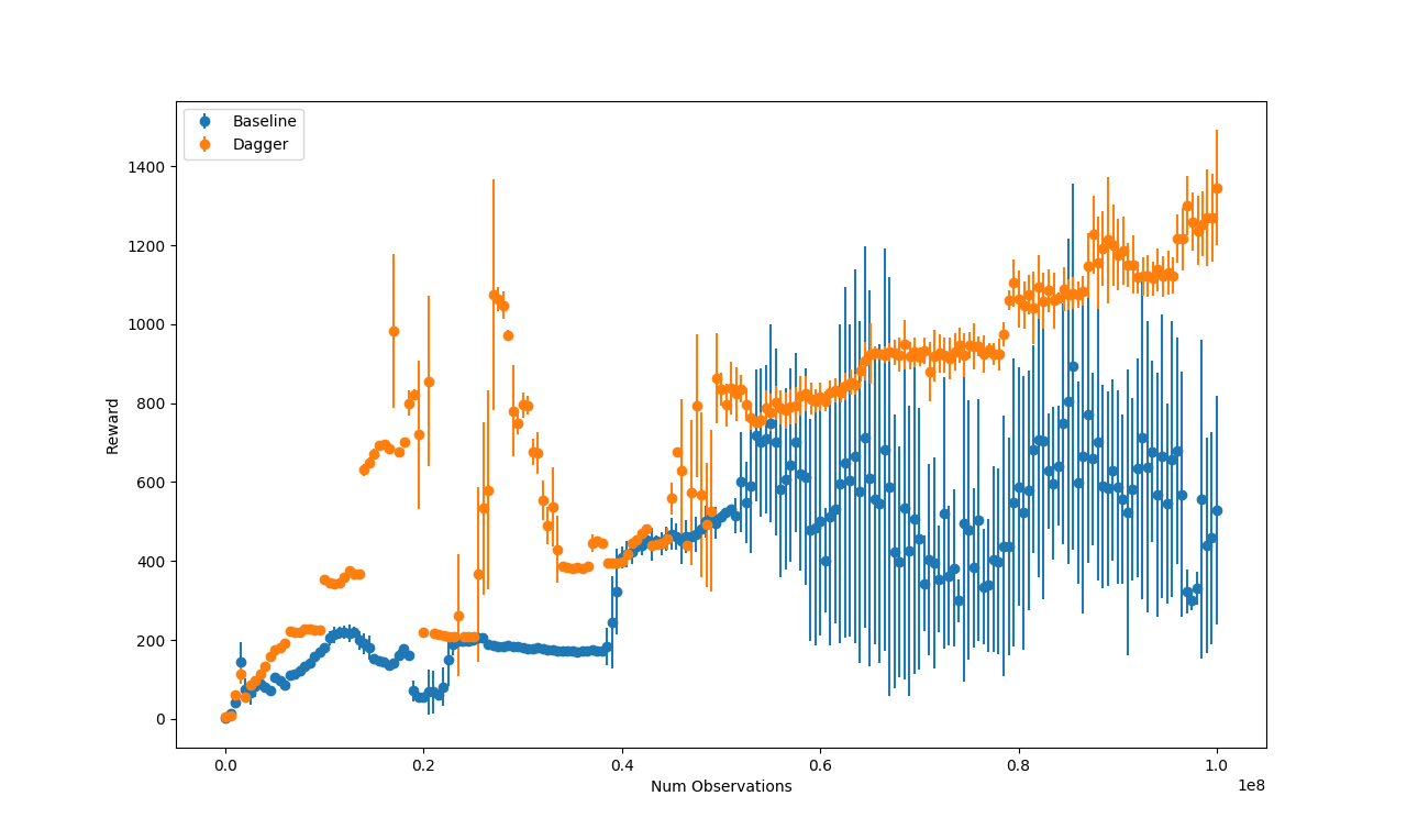
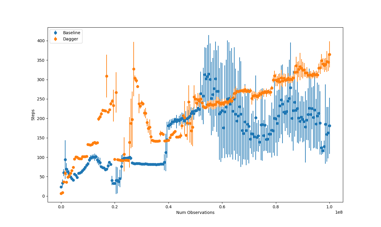
As seen the two graphs mirror each other (since the reward in this environment comes from staying upright while moving). The model trained with Dagger starts to have noticeable benefits about halfway through the training regime.

other

Some of the auxiliary code for loading the experts comes from the github repo for Berkeley’s Deep Reinforcement Learning course.

The code can be found on my GitHub.