intro

Convolutional neural networks are full of artifacts. Properly calibrated images of static (to the human eye) can therefore be strongly classified (>99.99% probability) as an image. Not knowing this paper existed, I set out to figure out if I could fool a CNN. Described are some of the techniques I used to do so, and how I generalized the approach to retrain the original CNN for a potential increase in model accuracy.

All code is freely available.

background

I use tensorflow (a symbolic programming language for Python) to build a convolutional neural network (CNN) for digit recognition. CNNs trained as pattern recognizers has a long history and the MNIST dataset is a canonical machine learning dataset. The training process is even covered in the tensorflow tutorials.

So once we have a fully trained CNN classifier, we have two questions:

1. How do we identify its artifacts? I.e. what are the intramodel relationships that results in spurious classifications?
2. Can we fix these artifacts?

process

overview

We first train a CNN on the MNIST dataset. Then we backwork inputs (using gradient descent on randomly intitialized inputs) to find strongly classified input images that look, to the human eye, nothing like the label as which they are classfied.

setup

First we build our model. See the build_model function in the proc_mnist.py.

params, x, y, layers = build_model(model_options, const_params=True)

Notice that x is now a variable that we will update and has dimensionality (batch_size, x_size, y_size).

cost

Next we need to build a cost to optimize in order to change x. To do this we will do two things simultaneously.

1. Maximize classification probability for some label l.
2. For each input/hidden layer, minimize the similarity between neuron activations at the layer (over the training data).

These two criteria suggest that we will get an input that is classified as label l but does not look like the other inputs the network was trained on.

getting values of neurons for training data

def compute_layers_fixed_label(data, label, x, layers, sess):

    labels = data.train.labels.argmax(1)
    mask = labels == label

    data_label = data.train.images[mask]

    layers_label = sess.run(layers, feed_dict={x: data_label})

    return layers_label

We evaluate this over all layers (except the output softmax layer) of the net.

layers_label = compute_layers_fixed_label(data, label, x, layers, sess)
layers_label = [tf.constant(a, name='layer{}_fixed_label'.format(idx)) for idx, a in enumerate(layers_label)]

building cost

At each layer the two costs are built with respect to these neuronal values at that layer across the training data. The costs at each layer can be broken into two parts.

1. reference_cost represents the similarity between patterns of activity for images being backworked and the patterns of activity across the training set. This will be used to select for images that “look” less like the training data to the net.
2. batch_cost represents the similarity between patterns of activity across all images in the batch.

def get_cost_from_layer(layer, layer_label, label):

    # For convolutional layers, layer has dimensionality (num_gen_examples, 28, 28, 1) and
    # layer_label has dimensionality (num_training_examples_label, 28, 28, 1)

    layer_name = layer.name.lower()

    # reference_dist_tensor is the tensor that represents the distance from generated images to the reference images
    # batch_dist_tensor is the tensor that represents the distance from generated images to other images in the batch
    reference_dist_tensor = tf.pow(layer - tf.expand_dims(layer_label, 1), 2)
    batch_dist_tensor = tf.pow(layer - tf.expand_dims(layer, 1), 2)

    if 'softmax' in layer_name:
        # Average all probabilities of guessing the wrong answer
        cost = 1 - layer[:, label]
        cost = tf.reduce_mean(cost)

        return cost,

    elif 'inputs' in layer_name or 'conv' in layer_name:
        # reference_dist_tensor has dimensionality (num_training_examples_label, num_gen_examples, 28, 28, 1)
        # Get the mean of the minimum distances of generated inputs to training examples of label
        reference_dist_tensor = tf.reduce_mean(reference_dist_tensor, reduction_indices=[2, 3, 4])

    elif 'fc' in layer_name:
        pass

    else:
        raise ValueError('Unknown layer type on layer %s', layer_name)

    reference_dist_tensor = tf.reduce_min(reference_dist_tensor, reduction_indices=[0])
    reference_dist_tensor = tf.reduce_mean(reference_dist_tensor)

    batch_dist_tensor = tf.reduce_mean(batch_dist_tensor)

    reference_cost = 1 / reference_dist_tensor
    batch_cost = 1 / batch_dist_tensor

    return reference_cost, batch_cost

The costs are weighted according to a user-defined weighting scheme. This allows for two things

1. layer_cost_coeffs enables costs at higher layers to be treated with greater importance than those at lower layers. Intuitively, this makes sense because features at higher layers represent greater levels of abstraction. So we would imagine that it would be better to find high level abstractions that are dissimilar to the high level abstractions representing data in the training set as this is more likely to correspond to meaningful dissimilarities to humans.
2. reference_cost_coeff represents the relative importance of inducing dissimilarities in the patterns of activity between examples from the batch and the training data. batch_cost_coeff represents the relative importance of inducing dissimilarities in the patterns of activity between examples inside the batch.*

* This was inspired by collisions found in the batch images. Relative increases in batch_cost_coeff motivate the system to find different artifacts of the classifier.

costs = [get_cost_from_layer(layer, layer_label, label) for layer, layer_label in zip(layers, layers_label)]
costs = [c for cost_tuple in costs for c in cost_tuple]

weights = np.outer(layer_cost_coeffs[: -1], [reference_cost_coeff, batch_cost_coeff]).flatten()
weights = np.append(weights, layer_cost_coeffs[-1])

costs = (costs * weights)

descent

Using gradient descent, we can manipulate images to minimize the cost function defined above.

optimize_input_layer = tf.train.AdamOptimizer(learning_rate=0.01).minimize(cost)

We set our convergence criteria as the minimum correct classification probability over a user defined value.

breaking out of local minima

Notice that in the softmax layer we count the cost as the mean misclassification probability across the batch. This means that many of the inputs in the batch may be strongly classified, but a few may not be able to escape the local minima they are in. To combat this, we will replace the most consistently misclassified inputs. If an input’s correct classification probability has been monotonically decreasing over num_mono_dec_saves saves (a save is just everytime the inputs are propagated forward to obtain classification probabilities) then it is reinitialized.

So with a mask m to denote which inputs need to be reinitialized, we can do the following:

input_vals[m] = np.random.rand(\*shape)
sess.run(x.assign(input_vals))

results

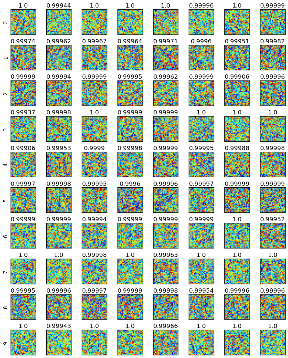
The minimum correct classification probability was set to 0.999. The reference_cost_coeff and batch_cost_coeff were each set to 1/2. layer_cost_coeffs were intialized in the log-space, for each non-softmax layer, to [1e-5, 1e-4, 1e-3, 1e-2]. The penalty at the softmax layer (for misclassification) was set to 10.

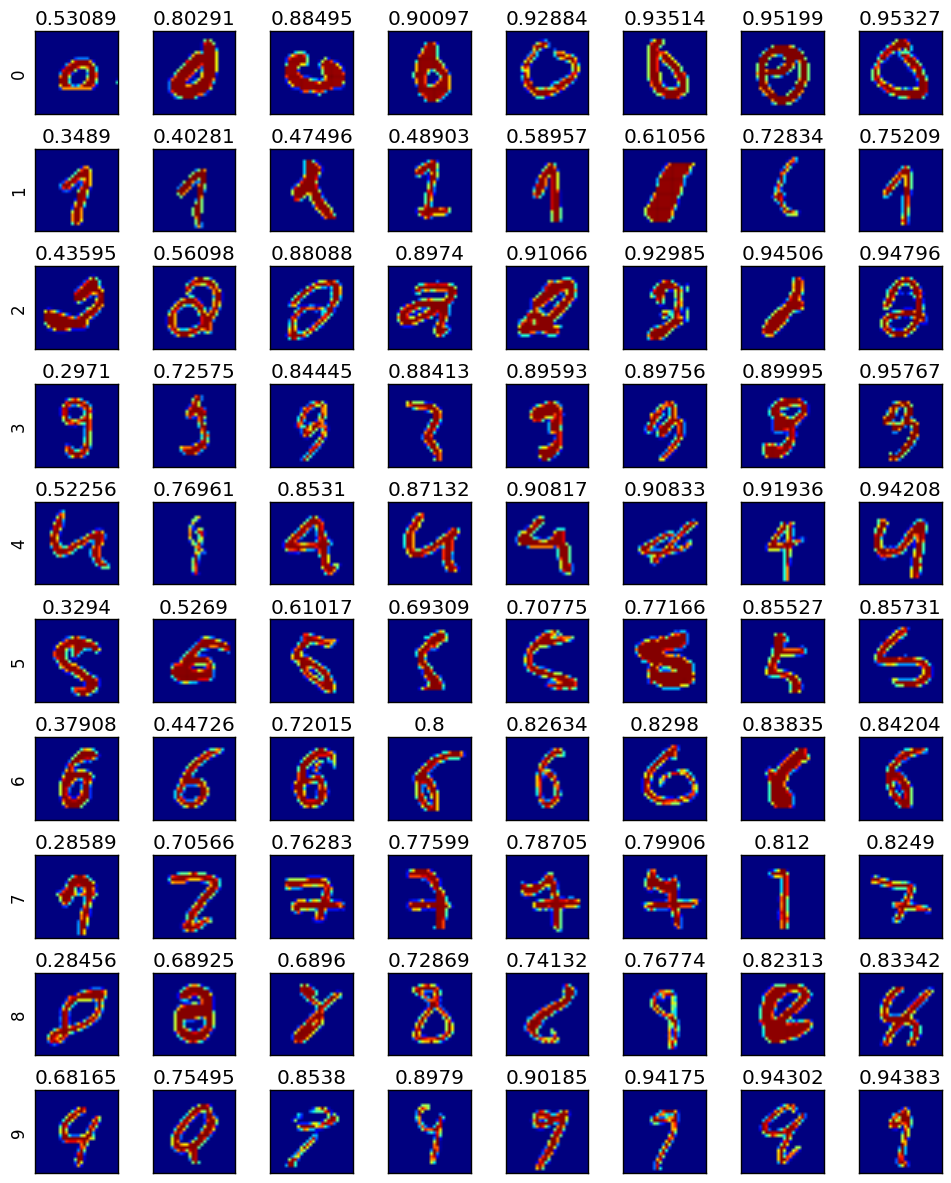
Here are eight input images, with probabilities of correct classification, that were put through this process for each of the 10 labels.

Here are eight images from the training set with associated probabilities of correct classification. These are the training examples that the net performs worst on.